Efficient alternate energy portable fuels are required to end our dependence on fossil fuels. Hydrogen holds the most promise in that reguard. Exploring the paths open for meeting the goal of energy independence is the object of this blog. Hopefully you will find it interesting and informative.
Thursday, October 6, 2011
Snake Oil Salesman or Simple Logic?
dF/dT=4(aFc+bFl+eFr), F=heat flux, T=Temperature, c=conduction, l=latent, r=radiative and a,b and e are constants of proportionality.
That is one amazingly powerful equation. All three heat fluxes have different properties but adhere to the same laws of physics. So all heat fluxes share the same basic relationship with temperature. Only their rates of flow vary with the method and media of propagation. They share the inverse square law. A general relativity of flux.
The first time I say this formula, which I have since modified with the coefficients, was on the Blackboard blog. It is the result of a paper in an obscure and controversial journal, Energy and Environment
If the journal had not been E&E and the debate on the internet, that formula would greatly simplify solutions to common mixed heat flux problems in the atmosphere.
The debate seems to center around the "implicit" Planck response of the atmosphere, but really should be centered around the coefficients, a, b and especially e, which I will call the Effective emissivity of radiative flux at the surface of the Earth.
That emissivity is generally e={dF/dT}/4 if a one degree change in temperature is due to a 3.3Wm-2 change in flux, the e=3.3/4=0.825 a unit less value, as 3.3 is the actual flow to temperature and 4 is the ideal flow to temperature. Extremely simple coefficient. For conduction, a, would be the ratio of actual flow to ideal flow, b, actual flow to ideal flow. Incredibly simple and elegant mathematics.
The e value is implicit it the climate science literature, it ranges from 0.61 to 1, ideal, with often 0.926, the value estimated by Stefan-Boltzman for a real black body since an ideal black body does not exist.
Update: The value for e is still an issue. Why? I have no clue, it is a benchmark value that can be determined in many ways, if you compare the approximate greenhouse temperature 33 to the approximate greenhouse energy flux 155, 155/33=4.7 Wm-2/K 4/4.7= 0.851 This is the initial value I determined for e which allows for the effective emissivity of the atmosphere. The surface though is still not a true black body, water has a very high emissivity of 0.99, but the average emissivity of all of Earth's surface is 0.967, which multiplied by the 0.851=.825. If anyone has a better estimate let me know.
The elegance can be seen in the Earth's atmosphere. Heat flux at the surface is divided into three forms, each with different characteristics of flow. Radiant heat for the surface does not uniformly interact with the atmosphere, only a portion e, interacts at differing spectral lines and intensities.
So a 100W/m-2 flux upward, with e=0.825 would produce a radiative interaction impact 82.5 W/m-2 in the atmosphere, down welling longwave radiation for some. An effective temperature for many others. This is the Greenhouse Effect, due to radiative flux. Conduction, convection and latent heat fluxes all contribute with differing impact as defined by their coefficients. This is so simple it should not require a proof. It is obvious in our physical world.
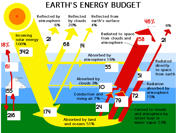
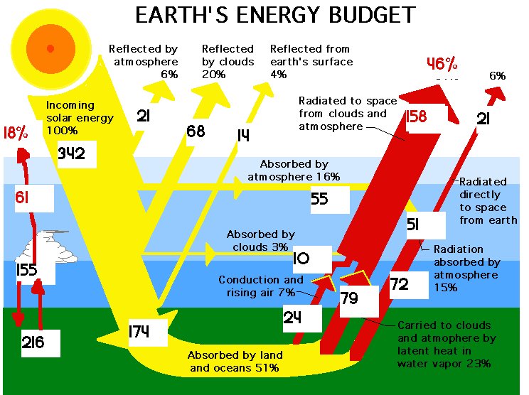
Using data from the NASA energy budget drawing, the atmosphere absorbs, 24 conductive, 78 latent and 51 radiative Wm-2 from the surface for a total of 153, the greenhouse effect. The atmosphere also absorbs 68 W/m-2 from the sun, the combined atmospheric effect is 153+68=221. All of these are absorbed values, eFr, not Fr needing adjustment. Since the solar is absorbed at different altitudes, its effect propagates according to the same simple inverse squared relationship. How hard do you really what to make nature?
http://ourhydrogeneconomy.blogspot.com/2011/10/call-for-mathematicians-greenhouse.html
Wednesday, October 5, 2011
A call for Mathematicians - The Greenhouse Effect, not so Simplified
This is extremely frustrating. Since there are errors in the math for the K&T drawing, I cannot explain the solution until I solve several other problems. So I am going to have to take much more time than I think is reasonable.
While Energy is Fungible, the Work is Not
Something so simple is so hard to explain.
Explaining the Kimoto equation unfortunately requires completely changing the way one looks at the atmospheric effect. In general, outgoing radiation balanced by down welling radiation of equal amounts have no net impact. The atmosphere is different. While the energy fluxes are just flows, they represent energy at a point in space and time. So while a surface flux may be matched, it has more impact at the surface. It creates more collisions in the denser environment. This is an increase in conductivity. So while two flows may pass, they are maintaining conductive conditions. Energy must be conserved, but the location of that energy is important.
In the atmosphere, there are changes in the type of energy flowing. There is latent heat from water warmed a the surface and carried aloft which does not lose its latent energy until it change phase. Conductive energy which is the number of collisions between molecules and radiant every which does not require a collision to release energy.
All three interact in the atmosphere until they revert to radiant energy and escape to space.
Each is better at transferring potential energy of a given type at a give efficiency. How easy it is to transfer heat from one boundary layer to another is extremely important. For example water is very efficient transferring energy via conduction to air that air is transferring energy to water. In an air to water heat exchanger, a conductive metal is used for the water and air boundary. Smooth tubes can be used on the water side without much loss of efficiency. On the air side, undulations are used to cause more turbulence in the air to increase the rate of collisions of the air molecules. On our oceans, heat flow from the surface increases with wave action and wind speed, more molecules contact the water's surface so more heat can be transferred. Water to air transfer of conductive heat is 1000 times more efficient that air to water, because the energy contain in every water molecule is much higher and the contact with other water molecules is much more efficient for transferring energy with in the water.
Air being orders of magnitude lower in density, takes longer to transfer energy between air molecules. Pure gases have different coefficients of heat transfer. Argon and Xenon are noble gases selected for their insulation qualities. Water vapor and carbon dioxide are not because they are better conductors. They are far from idea, but better
For example gases at atmospheric pressure separated by metal have heat transfer coefficients of 5 to 35 W/m^2K under pressure that changes to 100 to 500W/m^2K.
Under normal atmospheric conditions, water vapor and CO2 enhance the heat transfer because they can absorb energy both by conduction and through radiation. Under pressure they can transfer more and at a higher temperature they can transfer more than under lower temperature and pressure. The addition of more carbon dioxide increases the radiate energy absorbed, the number of collisions which increases the rate of conduction and increase the rate of evaporation. If there is a window for radiant heat transfer, some of this energy is transferred further from the water's surface which tends to decrease the rate of heat transfer because radiate heat transfer is not as efficient as conductive.
In the atmosphere, the adaptions of the Kimoto equation tells me, that while energy is fungible, the impact of the flows are very different, 24Wm-2 up of conductive flux is balance by 24Wm-2 down of radiative flux down from one point in the atmosphere, is not the same as 24Wm-2 up 100 meters and matched by a counter flux of 24Wm-2 at the TOA.
Below I was a brief derivation of the initial greenhouse effect. It is difficult to follow, because the assumptions, while valid are a bit unusual in the computer age. Now it is no longer brief.
For a temperature radiative flux relationship, dF/dT=4F/T This basic equation is part of the problem. while it is perfect for a radiative only solution it gets involve proving it can be used for a mixed heat flux solution. When I set the equation up for the Earth I get.
dF/dT= 4*(aFc + bFl +cFr)/T, a=conductive heat flow coefficient, b=latent heat flow coefficient and c=radiative heat flow coefficient aka emissivity. With the separate coefficients, this is totally valid, however with the proper valid assumptions I can make a and b disappear. And not by magic, by logic.
If dT/dt=0, i.e. it is in equilibrium with space and surface temperature does not change, then
Equilibrium can be assumed for a steady state, equilibrium may never truly exist, it is a numerical concept. It is very important that this equilibrium be understood. I am going to apply a radical impulse.
If the Earth was floating in space all by itself at a temperature of 288K and with no atmosphere, T=390W.m-2, aFc=0, dFl=0 and C=1 Fr=390 Do I have to explain how I got that? I hope not, with no atmosphere there would only be radiant heat loss.
Now you need a little imagination,
If we suddenly add an atmosphere, T=4*(aFc+bFl+0.825Fr), 0.825 is an impulse change in emissivity from 1 to 0.825, and following happens, aFc=24, bFl=76 and cFr=290 as it leaves the surface of the Earth. By selecting the approximate final value, I eliminate the need to solve three simultaneous equations.
Note: This value of 0.825 for the coefficient of Fr was carefully selected based on the current estimate of climate sensitivity. While there are many that may disagree it is valid, it simplifies the solution. If it is wrong, that will be obvious once we get to the final solution. I will try to clean up the methods I used to arrive at that value, but not until this stage has been simplified enough for others to understand.
By selecting the final values of aFc and bFl I am in effect assuming a solution for a and c. This is a little bit of mathematical trickery not common place any more. Since I am assuming that the responses of aFc and bFl are low and slow with respect to eFr, Fc and Fl would stabilize prior to Fr. Since the impulse is applied only to Fr via the change in emissivity and the stable values of Fc and Fl assumed correct, there would be insignificant harmonic interference with Fr's approach to the new equilibrium state. This is a very effective simplification.
Okay, a little more imagination, once the surface and the atmosphere reach a steady state, equilibrium, for the briefest moment in time, we get aFc=24, bFl=76 and c becomes 0.825 which changes cFr to 0.825*290=239.5, so for that moment all hell breaks loose. The Earth would attempt to maintain the 390Wm-2 total flux, it would overshoot, and gradually seek equilibrium. Before it finds equilibrium, the atmospheric resistance to flux with the impulse change in emissivity would over shot a peak value. Knowing the final value at the TOA, 237 and the final temperature and flux at the surface, we can determine the initial green house response by artificial selecting a high but very close to reality, impulse flux from the surface. This must be trickier that I thought because no one understands this trick. Then,
T=4(aFc+bFc+cFr)+4GHe, that should be fairly simple to follow, do I need to expand that? Since I will be solving for the impulse value of GHe, I have to modify the equation. Should not be that hard to follow.
4GHe=T-4(aFc+bFc+cFr)
GHe=(T-4(aFc+bFc+cFr))/4
So the initial Greenhouse effect(GHe) is,
GHe=(288-4*(24+76+239.5)/4 = (288-4*339.5)/4 = -267.5
I selected 239.5 for convenience. I could have picked 400 or infinity, but the closer it is to reality the more information we can obtain.
That is the end of the first moment in time, a sudden impulse to a BB in equilibrium at the average temperature of Earth. Still no sun, that will be at the end.
GHe=-267.5 which has to be matched by Outgoing Longwave Radiation (OLR) in the second moment in time for the surface to regain equilibrium. The assumption of equilibrium at the surface is critical. The approximate equilibrium value at the TOA will be assumed for this stage.
390-267=122.5, the initial surface response to the GHe.
Had I selected a higher value for Fr, both the initial -267.5 and the resulting value 122.5 would have been different, but proportionally different. That is the trick by selecting 239.5 up to 390 I avoid the confusion of the sign change. The sign of GHe is very important, the value after subtracting from 390 not so important because we know that it will return to 390. It is the proportion and sign of GHe that matter. In the next step you can see why I chose a value close to the equilibrium value of Fr.
As the surface of the Earth obtains equilibrium with the atmosphere,
Surface (24+76+239.5+122.5)=462 is the initial peak radiation which will decay as equilibrium is approached. -267.5 is the initial value of the greenhouse effect which will decay as equilibrium is approached. These are impulse conditions. At the TOA, the flux has dropped to near zero and will stabilize to a value of 237Wm-2.
As you can see the peak 462 is a manageable number. It is a totally fictitious number, but it is proportional to the -271 GHe impulse which is also fictitious. As long as they are proportional, greater that the final value and the signs are correct, these values will work. But, since I selected 239.5 for the value, which is steady state, there is some meaning in -271 and 462.
At this point we release Temperature so that it actually change. The surface will reduce its emitted radiation by 462-390=72Wm-2 The radiation at the top of the atmosphere will decay to 239.5Wm-2. This is the start of the third layer solution. By selecting 239.5, I get 462 peak at the surface minus 271 in the atmosphere. 462+(-271)=191 at the TOA. The TOA has to increase to 239.5 and 462 has to decrease to 390. GHe cannot increase if 462 is decreasing and 191 is increasing. So both have to decay, or reduce in magnitude, to a stable value while TOA is increasing. This must be part of my trick that is very hard to f0llow.
At the surface, 462 decreases as 122.5 decays to 72 yielding 50.5, the amount of radiation absorbed by the atmosphere. The GHe -267.5 proportionally with the 122.5 decays to -267.5 + 50.5 = -217 The 50.5 is a verification of the method, but not if you were using the Trenberth values. 51 is the determined by NASA, 50.5 tends to confirm their calculations.
This final step may be difficult, but not so bad if you have followed me so far.
There is still no sun in the sky, this is the third moment in the existence of the atmosphere. With no solar input at all, the problem is super simplified. This equilibrium condition would exist on for the briefest period of time.
The TOA value of 237 is assumed to be the momentary equilibrium value. Trenberth added the 72 to 267.5 to get 339 and then decayed that to 321, 339-321=18, the amount he mistakenly has for atmospheric absorption.
In order to solve for the solar input, I have to use the same methods, only the it is not really needed. Since the equilibrium values are very close to the real world values, adding the sun only requires minor accounting to resolve the atmospheric balance. Think of should I let the surface flux decrease to 390 minus any small value, then slowly increase the solar values to maintain the 390. Instead of adding an impulse, the slow matching input maintains the surface balance and the TOA balance, then it is just minor accounting to solve the atmospheric balance. Since the upeard flux does not change, the down welling will not change since it is created by resistance to outgoing flow. The values selected for Fc and Fl are based on the steady state with solar, so only the upper troposphere needs to be tweaked.
Setting up this solution was most of the battle. It took me a while to confirm that 0.825 was a valid estimate, I had to determine a reasonable estimate of the DWR from comparing both K&T drawings to the NASA, I had to basically solve the problem before I could solve the problem. So this is not the best or only way, it is only A way.
Now I have confirmed the Trenberth error several ways, but it is difficult to unseat the champion. Unfortunately, there are probably not many people that can appreciate the simple elegance of this mathematical trickery. Unfortunately, this method will probably not be accepted even though all the assumptions are valid, because they push the limits pretty severely. Until this first step is understood and at least somewhat accepted I cannot advance to calculating climate sensitivity with greater accuracy using the simple formula dF/dT=4F/T with the proper coefficients.
I think I will call this proof by discovery of error. If you look closely at the K&T you should confirm the DWR and atmospheric absorption errors which amplify each other in opposite directions. In the old K&T, 26 was the atmospheric absorption of net OLR and the new it is 18 in the old, both require a little snooping to decipher, but they are there. 51, or 50.5 calculated here, appear to be the appropriate values. The correct DWR value is fairly obvious also in the NASA with a little looking. If that is not enough, Angstrom's turn of the 20th century estimate was closer than the K&T drawing. Check Eli Rabbet's blog.
I would like to thank Fred Moolton for helping me figure out what was so hard to understand.
While Energy is Fungible, the Work is Not
Something so simple is so hard to explain.
Explaining the Kimoto equation unfortunately requires completely changing the way one looks at the atmospheric effect. In general, outgoing radiation balanced by down welling radiation of equal amounts have no net impact. The atmosphere is different. While the energy fluxes are just flows, they represent energy at a point in space and time. So while a surface flux may be matched, it has more impact at the surface. It creates more collisions in the denser environment. This is an increase in conductivity. So while two flows may pass, they are maintaining conductive conditions. Energy must be conserved, but the location of that energy is important.
In the atmosphere, there are changes in the type of energy flowing. There is latent heat from water warmed a the surface and carried aloft which does not lose its latent energy until it change phase. Conductive energy which is the number of collisions between molecules and radiant every which does not require a collision to release energy.
All three interact in the atmosphere until they revert to radiant energy and escape to space.
Each is better at transferring potential energy of a given type at a give efficiency. How easy it is to transfer heat from one boundary layer to another is extremely important. For example water is very efficient transferring energy via conduction to air that air is transferring energy to water. In an air to water heat exchanger, a conductive metal is used for the water and air boundary. Smooth tubes can be used on the water side without much loss of efficiency. On the air side, undulations are used to cause more turbulence in the air to increase the rate of collisions of the air molecules. On our oceans, heat flow from the surface increases with wave action and wind speed, more molecules contact the water's surface so more heat can be transferred. Water to air transfer of conductive heat is 1000 times more efficient that air to water, because the energy contain in every water molecule is much higher and the contact with other water molecules is much more efficient for transferring energy with in the water.
Air being orders of magnitude lower in density, takes longer to transfer energy between air molecules. Pure gases have different coefficients of heat transfer. Argon and Xenon are noble gases selected for their insulation qualities. Water vapor and carbon dioxide are not because they are better conductors. They are far from idea, but better
For example gases at atmospheric pressure separated by metal have heat transfer coefficients of 5 to 35 W/m^2K under pressure that changes to 100 to 500W/m^2K.
Under normal atmospheric conditions, water vapor and CO2 enhance the heat transfer because they can absorb energy both by conduction and through radiation. Under pressure they can transfer more and at a higher temperature they can transfer more than under lower temperature and pressure. The addition of more carbon dioxide increases the radiate energy absorbed, the number of collisions which increases the rate of conduction and increase the rate of evaporation. If there is a window for radiant heat transfer, some of this energy is transferred further from the water's surface which tends to decrease the rate of heat transfer because radiate heat transfer is not as efficient as conductive.
In the atmosphere, the adaptions of the Kimoto equation tells me, that while energy is fungible, the impact of the flows are very different, 24Wm-2 up of conductive flux is balance by 24Wm-2 down of radiative flux down from one point in the atmosphere, is not the same as 24Wm-2 up 100 meters and matched by a counter flux of 24Wm-2 at the TOA.
Below I was a brief derivation of the initial greenhouse effect. It is difficult to follow, because the assumptions, while valid are a bit unusual in the computer age. Now it is no longer brief.
For a temperature radiative flux relationship, dF/dT=4F/T This basic equation is part of the problem. while it is perfect for a radiative only solution it gets involve proving it can be used for a mixed heat flux solution. When I set the equation up for the Earth I get.
dF/dT= 4*(aFc + bFl +cFr)/T, a=conductive heat flow coefficient, b=latent heat flow coefficient and c=radiative heat flow coefficient aka emissivity. With the separate coefficients, this is totally valid, however with the proper valid assumptions I can make a and b disappear. And not by magic, by logic.
If dT/dt=0, i.e. it is in equilibrium with space and surface temperature does not change, then
Equilibrium can be assumed for a steady state, equilibrium may never truly exist, it is a numerical concept. It is very important that this equilibrium be understood. I am going to apply a radical impulse.
If the Earth was floating in space all by itself at a temperature of 288K and with no atmosphere, T=390W.m-2, aFc=0, dFl=0 and C=1 Fr=390 Do I have to explain how I got that? I hope not, with no atmosphere there would only be radiant heat loss.
Now you need a little imagination,
If we suddenly add an atmosphere, T=4*(aFc+bFl+0.825Fr), 0.825 is an impulse change in emissivity from 1 to 0.825, and following happens, aFc=24, bFl=76 and cFr=290 as it leaves the surface of the Earth. By selecting the approximate final value, I eliminate the need to solve three simultaneous equations.
Note: This value of 0.825 for the coefficient of Fr was carefully selected based on the current estimate of climate sensitivity. While there are many that may disagree it is valid, it simplifies the solution. If it is wrong, that will be obvious once we get to the final solution. I will try to clean up the methods I used to arrive at that value, but not until this stage has been simplified enough for others to understand.
By selecting the final values of aFc and bFl I am in effect assuming a solution for a and c. This is a little bit of mathematical trickery not common place any more. Since I am assuming that the responses of aFc and bFl are low and slow with respect to eFr, Fc and Fl would stabilize prior to Fr. Since the impulse is applied only to Fr via the change in emissivity and the stable values of Fc and Fl assumed correct, there would be insignificant harmonic interference with Fr's approach to the new equilibrium state. This is a very effective simplification.
Okay, a little more imagination, once the surface and the atmosphere reach a steady state, equilibrium, for the briefest moment in time, we get aFc=24, bFl=76 and c becomes 0.825 which changes cFr to 0.825*290=239.5, so for that moment all hell breaks loose. The Earth would attempt to maintain the 390Wm-2 total flux, it would overshoot, and gradually seek equilibrium. Before it finds equilibrium, the atmospheric resistance to flux with the impulse change in emissivity would over shot a peak value. Knowing the final value at the TOA, 237 and the final temperature and flux at the surface, we can determine the initial green house response by artificial selecting a high but very close to reality, impulse flux from the surface. This must be trickier that I thought because no one understands this trick. Then,
T=4(aFc+bFc+cFr)+4GHe, that should be fairly simple to follow, do I need to expand that? Since I will be solving for the impulse value of GHe, I have to modify the equation. Should not be that hard to follow.
4GHe=T-4(aFc+bFc+cFr)
GHe=(T-4(aFc+bFc+cFr))/4
So the initial Greenhouse effect(GHe) is,
GHe=(288-4*(24+76+239.5)/4 = (288-4*339.5)/4 = -267.5
I selected 239.5 for convenience. I could have picked 400 or infinity, but the closer it is to reality the more information we can obtain.
That is the end of the first moment in time, a sudden impulse to a BB in equilibrium at the average temperature of Earth. Still no sun, that will be at the end.
GHe=-267.5 which has to be matched by Outgoing Longwave Radiation (OLR) in the second moment in time for the surface to regain equilibrium. The assumption of equilibrium at the surface is critical. The approximate equilibrium value at the TOA will be assumed for this stage.
390-267=122.5, the initial surface response to the GHe.
Had I selected a higher value for Fr, both the initial -267.5 and the resulting value 122.5 would have been different, but proportionally different. That is the trick by selecting 239.5 up to 390 I avoid the confusion of the sign change. The sign of GHe is very important, the value after subtracting from 390 not so important because we know that it will return to 390. It is the proportion and sign of GHe that matter. In the next step you can see why I chose a value close to the equilibrium value of Fr.
As the surface of the Earth obtains equilibrium with the atmosphere,
Surface (24+76+239.5+122.5)=462 is the initial peak radiation which will decay as equilibrium is approached. -267.5 is the initial value of the greenhouse effect which will decay as equilibrium is approached. These are impulse conditions. At the TOA, the flux has dropped to near zero and will stabilize to a value of 237Wm-2.
As you can see the peak 462 is a manageable number. It is a totally fictitious number, but it is proportional to the -271 GHe impulse which is also fictitious. As long as they are proportional, greater that the final value and the signs are correct, these values will work. But, since I selected 239.5 for the value, which is steady state, there is some meaning in -271 and 462.
At this point we release Temperature so that it actually change. The surface will reduce its emitted radiation by 462-390=72Wm-2 The radiation at the top of the atmosphere will decay to 239.5Wm-2. This is the start of the third layer solution. By selecting 239.5, I get 462 peak at the surface minus 271 in the atmosphere. 462+(-271)=191 at the TOA. The TOA has to increase to 239.5 and 462 has to decrease to 390. GHe cannot increase if 462 is decreasing and 191 is increasing. So both have to decay, or reduce in magnitude, to a stable value while TOA is increasing. This must be part of my trick that is very hard to f0llow.
At the surface, 462 decreases as 122.5 decays to 72 yielding 50.5, the amount of radiation absorbed by the atmosphere. The GHe -267.5 proportionally with the 122.5 decays to -267.5 + 50.5 = -217 The 50.5 is a verification of the method, but not if you were using the Trenberth values. 51 is the determined by NASA, 50.5 tends to confirm their calculations.
This final step may be difficult, but not so bad if you have followed me so far.
There is still no sun in the sky, this is the third moment in the existence of the atmosphere. With no solar input at all, the problem is super simplified. This equilibrium condition would exist on for the briefest period of time.
The TOA value of 237 is assumed to be the momentary equilibrium value. Trenberth added the 72 to 267.5 to get 339 and then decayed that to 321, 339-321=18, the amount he mistakenly has for atmospheric absorption.
In order to solve for the solar input, I have to use the same methods, only the it is not really needed. Since the equilibrium values are very close to the real world values, adding the sun only requires minor accounting to resolve the atmospheric balance. Think of should I let the surface flux decrease to 390 minus any small value, then slowly increase the solar values to maintain the 390. Instead of adding an impulse, the slow matching input maintains the surface balance and the TOA balance, then it is just minor accounting to solve the atmospheric balance. Since the upeard flux does not change, the down welling will not change since it is created by resistance to outgoing flow. The values selected for Fc and Fl are based on the steady state with solar, so only the upper troposphere needs to be tweaked.
Setting up this solution was most of the battle. It took me a while to confirm that 0.825 was a valid estimate, I had to determine a reasonable estimate of the DWR from comparing both K&T drawings to the NASA, I had to basically solve the problem before I could solve the problem. So this is not the best or only way, it is only A way.
Now I have confirmed the Trenberth error several ways, but it is difficult to unseat the champion. Unfortunately, there are probably not many people that can appreciate the simple elegance of this mathematical trickery. Unfortunately, this method will probably not be accepted even though all the assumptions are valid, because they push the limits pretty severely. Until this first step is understood and at least somewhat accepted I cannot advance to calculating climate sensitivity with greater accuracy using the simple formula dF/dT=4F/T with the proper coefficients.
I think I will call this proof by discovery of error. If you look closely at the K&T you should confirm the DWR and atmospheric absorption errors which amplify each other in opposite directions. In the old K&T, 26 was the atmospheric absorption of net OLR and the new it is 18 in the old, both require a little snooping to decipher, but they are there. 51, or 50.5 calculated here, appear to be the appropriate values. The correct DWR value is fairly obvious also in the NASA with a little looking. If that is not enough, Angstrom's turn of the 20th century estimate was closer than the K&T drawing. Check Eli Rabbet's blog.
I would like to thank Fred Moolton for helping me figure out what was so hard to understand.
A better Cartoon?
Willis Eschenbach is a climate change skeptic with a clue. He has modified the Kiehl and Trenberth cartoon to allow for layers. Imagine that? Since he has done that, I don't have to. I am going to borrow his version, hopefully without being sued, to compare the things that I found out in the Back to Baking Bacon Bread post.
Willis added a tropopause break to separate the troposphere from the upper atmosphere. Excellent move! The values on his drawing are true to the more recent K&T cartoon. In analysis I did I used the older version.
In the post I did before I found that a ratio of temperature change from the atmosphere should equal the ratio of the energy flux change in the atmosphere. The flux at the surface 392Wm-2, is supposed to be the energy radiated by a black body at a temperature of 288K degrees. This flux would assume the application of emissivity of the planet and is based on the average temperature. The calculated temperature at the Top of the Atmosphere is 255K degrees for a radiant flux of 237Wm-2. Note that this value is slightly larger than the 235 on their old cartoon and slight lower than the general estimate of 240Wm-2. The difference between 392 and 237 is 155Wm-2 just as it was in the older cartoon. The actually average surface temperature is fairly accurately estimated at 288K and the flux at the TOA is fairly accurately measurable along with the temperature of 255 degrees K. the largest uncertainty appears to be the actual flux rate at the surface. Measuring that flux rate is extremely complicated and the accuracy of the measuring instruments is roughly 2% of the range. For a pure black body, the uncertainty in the emissivity is very small. For a gray body, the emissivity is a bit more debatable, but generally thought to be fairly accurate. The issue is that 288-255=33 has to have a consistent ratio with range of flux change in the atmosphere. So 33/288-30 = 1 and 155/(392-237) = 1 should have a direct relationship by the equation dF/dT=4F/T or a change in T=4F. The estimated sensitivity of the Earth surface to a doubling of CO2 is related to the change in flux by 3.7 1T=3.7F in a change. 3.7 is close to 4, 3.7/4=0.925, which is the estimated emissivity of the atmosphere. Pretty simple. However, in my previous post, the emissivity of the atmosphere appears to be 0.85 and not 0.925. 0.85/0.925=0.92 or 8% less than estimated. That difference could lead to a +/-8% error where contrasting errors could be 16%. Complimentary errors would negate.
Or vice versa depending on how you look at it.
In the flux ratio, since its change is 4 times that of temperature, that error would be multiplied by a factor of 4. So it would only take a relatively small error measuring temperature to result in a fairly large error in calculated flux. Since flux is not easily measured, it makes the use of calculating flux very common. A small error in flux measured would result in a smaller error of temperature calculated. So it would be easy for me or anyone else to have big issues if temperature measurement is wrong and the effective emissivity is off by 8 percent. The best estimate for effective emissivity (e)is 0.85, and 3.7Wm=-2 is estimate to cause a 1.2K increase in temperature, we can arraign the dT=3.7/(0.825*4)=3.7/3.3=1.12K and see that 1.12/1.2=93% of the estimated warming. Effective emissivity is however the variable to be changed causing the increase change in flux. If the Earth were a perfect black body,e=1, so the change in flux from the surface would be 155Wm-2. If the Earth were a regular back body, e=0.926, then the flux change from the surface would be would be 143.5Wm-2, so the surface flux would be 237+143.5=380Wm-2 Well, the Earth's surface is closer to a black body than the atmosphere. A one degree increase in the surface temperature would produce an increased flux of .926*4=3.7 Wm-2. The Earth though is mainly water and the emissivity of water is 0.99, so a one degree increase in the temperature of the oceans would cause a 4Wm-2 increase in flux. Conversely, one degree increase in surface air temperature would only cause a 3.3/4=0.825 degree increase in the ocean temperature, That increase in flux would produce 3.7/3.3=1.12K increase in temperature.
The ocean air interface is the greenhouse effect, radiant heat leaving the ocean surface at 100Wm-2 is restricted to 82 Wm-2 when it hits the atmosphere, conductive heat from water flows at 10,000Wm-2 and is restricted to 100Wm-2, latent heat from the ocean is restricted by the relative humidity of the air. All three modes of heat transport are bottle necked at the surface. Chop created by winds increase the cooling of the oceans, but not the absorption of energy. The Earth's real thermostat.
So looking at the K&T drawing for the surface, Fc=24, Fl=76 and Fr=392-24-76= 292 Where Fc is the thermals heat loss, Fl is the latent heat loss and Fr is the radiant heat loss. Fr though is balanced by down welling radiation created by the radiative bottleneck change from emissivity nearly 1 to 0.825. At the surface we have 292*.825=239Wm-2 leaving, 292-239=53Wm-2, which is the value that should be used for radiative absorption by the atmosphere, not the 18 implied by the 339 in and 321out for the troposphere shown of the drawing. The total of all the downwelling created by Fc, Fl and Fr is 392-239=153Wm-2. Since I undoubtedly had some rounding errors, 155Wm-2 is close enough for government work. So dF/dT=4(cFc+lFl+eFr)/T is perfectly valid at the surface, as long as the coefficients,c and l are small in comparison to e.
Update: I fixed a small error and missed one calculation. 239-155=84 which would be Frnet or the net radiative flux through the atmosphere from the surface proper. 51 of that should be absorbed in the troposphere and 33 radiated to space. Since water as a liquid and solid in the atmosphere can radiate in the atmospheric window, that should be shown at the top of the troposphere
There appears to be an issue with the K&T drawing right at the surface. DWR should be between 206 and 239 not 321.
Willis added a tropopause break to separate the troposphere from the upper atmosphere. Excellent move! The values on his drawing are true to the more recent K&T cartoon. In analysis I did I used the older version.
In the post I did before I found that a ratio of temperature change from the atmosphere should equal the ratio of the energy flux change in the atmosphere. The flux at the surface 392Wm-2, is supposed to be the energy radiated by a black body at a temperature of 288K degrees. This flux would assume the application of emissivity of the planet and is based on the average temperature. The calculated temperature at the Top of the Atmosphere is 255K degrees for a radiant flux of 237Wm-2. Note that this value is slightly larger than the 235 on their old cartoon and slight lower than the general estimate of 240Wm-2. The difference between 392 and 237 is 155Wm-2 just as it was in the older cartoon. The actually average surface temperature is fairly accurately estimated at 288K and the flux at the TOA is fairly accurately measurable along with the temperature of 255 degrees K. the largest uncertainty appears to be the actual flux rate at the surface. Measuring that flux rate is extremely complicated and the accuracy of the measuring instruments is roughly 2% of the range. For a pure black body, the uncertainty in the emissivity is very small. For a gray body, the emissivity is a bit more debatable, but generally thought to be fairly accurate. The issue is that 288-255=33 has to have a consistent ratio with range of flux change in the atmosphere. So 33/288-30 = 1 and 155/(392-237) = 1 should have a direct relationship by the equation dF/dT=4F/T or a change in T=4F. The estimated sensitivity of the Earth surface to a doubling of CO2 is related to the change in flux by 3.7 1T=3.7F in a change. 3.7 is close to 4, 3.7/4=0.925, which is the estimated emissivity of the atmosphere. Pretty simple. However, in my previous post, the emissivity of the atmosphere appears to be 0.85 and not 0.925. 0.85/0.925=0.92 or 8% less than estimated. That difference could lead to a +/-8% error where contrasting errors could be 16%. Complimentary errors would negate.
Or vice versa depending on how you look at it.
In the flux ratio, since its change is 4 times that of temperature, that error would be multiplied by a factor of 4. So it would only take a relatively small error measuring temperature to result in a fairly large error in calculated flux. Since flux is not easily measured, it makes the use of calculating flux very common. A small error in flux measured would result in a smaller error of temperature calculated. So it would be easy for me or anyone else to have big issues if temperature measurement is wrong and the effective emissivity is off by 8 percent. The best estimate for effective emissivity (e)is 0.85, and 3.7Wm=-2 is estimate to cause a 1.2K increase in temperature, we can arraign the dT=3.7/(0.825*4)=3.7/3.3=1.12K and see that 1.12/1.2=93% of the estimated warming. Effective emissivity is however the variable to be changed causing the increase change in flux. If the Earth were a perfect black body,e=1, so the change in flux from the surface would be 155Wm-2. If the Earth were a regular back body, e=0.926, then the flux change from the surface would be would be 143.5Wm-2, so the surface flux would be 237+143.5=380Wm-2 Well, the Earth's surface is closer to a black body than the atmosphere. A one degree increase in the surface temperature would produce an increased flux of .926*4=3.7 Wm-2. The Earth though is mainly water and the emissivity of water is 0.99, so a one degree increase in the temperature of the oceans would cause a 4Wm-2 increase in flux. Conversely, one degree increase in surface air temperature would only cause a 3.3/4=0.825 degree increase in the ocean temperature, That increase in flux would produce 3.7/3.3=1.12K increase in temperature.
The ocean air interface is the greenhouse effect, radiant heat leaving the ocean surface at 100Wm-2 is restricted to 82 Wm-2 when it hits the atmosphere, conductive heat from water flows at 10,000Wm-2 and is restricted to 100Wm-2, latent heat from the ocean is restricted by the relative humidity of the air. All three modes of heat transport are bottle necked at the surface. Chop created by winds increase the cooling of the oceans, but not the absorption of energy. The Earth's real thermostat.
So looking at the K&T drawing for the surface, Fc=24, Fl=76 and Fr=392-24-76= 292 Where Fc is the thermals heat loss, Fl is the latent heat loss and Fr is the radiant heat loss. Fr though is balanced by down welling radiation created by the radiative bottleneck change from emissivity nearly 1 to 0.825. At the surface we have 292*.825=239Wm-2 leaving, 292-239=53Wm-2, which is the value that should be used for radiative absorption by the atmosphere, not the 18 implied by the 339 in and 321out for the troposphere shown of the drawing. The total of all the downwelling created by Fc, Fl and Fr is 392-239=153Wm-2. Since I undoubtedly had some rounding errors, 155Wm-2 is close enough for government work. So dF/dT=4(cFc+lFl+eFr)/T is perfectly valid at the surface, as long as the coefficients,c and l are small in comparison to e.
Update: I fixed a small error and missed one calculation. 239-155=84 which would be Frnet or the net radiative flux through the atmosphere from the surface proper. 51 of that should be absorbed in the troposphere and 33 radiated to space. Since water as a liquid and solid in the atmosphere can radiate in the atmospheric window, that should be shown at the top of the troposphere
There appears to be an issue with the K&T drawing right at the surface. DWR should be between 206 and 239 not 321.
Trenberth, Monckton and Lucia - Are They missing the Heat?
In my last post Back to Baking Bacon Bread, the pork fat must have stimulated my brain or killed a few extra brain cells, not sure which. Anyway, in my pork fat euphoria, it appears I have located a missing 22Wm-2 of heat. Because of the sensitivity of errors, it is not all that easy to find out how much heat is missing versus some just misplaced.
However, since it looks like the flux generated by the greenhouse effect is 133 and not 155, there is probably a slight error in estimating the effective emissivity of the Earth's atmosphere, the planet itself or both. That is not only likely, but probable. The question would be how much would it effect the overall estimation of the change in forcing due to a doubling of CO2? Hummm?
I am not sure how to go directly to the answer. I can start by using the 133 instead of 155 just to see what that may do.
Back to my new favorite formula, dF/dT=4F/T and the ratio Tge/(288-255)=Fge/(390-235), the 390, Fs(urface)-235, Ftoa equals 155, but that does not include the effective emissivity of the atmosphere. Effective emissivity would be 133/155=0.85, which is much lower than typically assumed. So modifying the ratio, 0.85*(Fge)/0.85(Fs-Ftoa), to allow for this emissivity value we have T/33=0.85Fge/133. Since we are solving for an unknown temperature change due to 2xCO2 we have, dTge=dFge*Tge/4Fge=0.85*(3.7*33)/(4*133)=0.195, so for a 3.7Wm-2 change in forcing, 0.72 degree K change. That is a considerably smaller amount than the 1 estimated, a lot smaller that the 1.2 often estimated and one hellava lot less than the 1.5 estimate by some. So I think it is worth looking into a bit.
The nuts of the matter is that warming is likely over estimated by up to 15%, 85% of 3C is 2.55 Degrees, which purely by chance I am sure, agrees nicely with most of the recent estimates of sensitivity and is just about how much the models are over estimating the impact of global warming.
Could it be the MISSING HEAT?
However, since it looks like the flux generated by the greenhouse effect is 133 and not 155, there is probably a slight error in estimating the effective emissivity of the Earth's atmosphere, the planet itself or both. That is not only likely, but probable. The question would be how much would it effect the overall estimation of the change in forcing due to a doubling of CO2? Hummm?
I am not sure how to go directly to the answer. I can start by using the 133 instead of 155 just to see what that may do.
Back to my new favorite formula, dF/dT=4F/T and the ratio Tge/(288-255)=Fge/(390-235), the 390, Fs(urface)-235, Ftoa equals 155, but that does not include the effective emissivity of the atmosphere. Effective emissivity would be 133/155=0.85, which is much lower than typically assumed. So modifying the ratio, 0.85*(Fge)/0.85(Fs-Ftoa), to allow for this emissivity value we have T/33=0.85Fge/133. Since we are solving for an unknown temperature change due to 2xCO2 we have, dTge=dFge*Tge/4Fge=0.85*(3.7*33)/(4*133)=0.195, so for a 3.7Wm-2 change in forcing, 0.72 degree K change. That is a considerably smaller amount than the 1 estimated, a lot smaller that the 1.2 often estimated and one hellava lot less than the 1.5 estimate by some. So I think it is worth looking into a bit.
The nuts of the matter is that warming is likely over estimated by up to 15%, 85% of 3C is 2.55 Degrees, which purely by chance I am sure, agrees nicely with most of the recent estimates of sensitivity and is just about how much the models are over estimating the impact of global warming.
Could it be the MISSING HEAT?
Tuesday, October 4, 2011
Back to Baking Bacon Bread
It is crusty roll fit for my crusty role.
Update: In case Fred show up, To use ratio and proportion correctly in this problem the 33C greenhouse effect would need to be equal to Surface radiation minus TOA radiation divide by four. 155/4=38.7 so either relationship in the equation is wrong, 33 is wrong or 155 is wrong, my money is on the 155.
Just in case you are wondering, the emissivity estimate of 0.926 only accounts for part of the difference, 143.5wm-2, there is still nearly 10 Wm-2 missing.
In the Monckton-Lucia online debate I am a non-combatant, I really don't care. I was curious if there was any justification for the linear approximation of flux versus temperature. Not only is there justification, there are several ways of using that approximation, with some pitfalls for the unwary. I will leave those issues to others. The one equation used was dF/dT=4F/T, so if I am going to use simple ratio and proportion to calculate a change in one relative to the other, it is a piece of cake. But is it valid with a mix of heat fluxes, latent thermal(sensible I prefer) and radiant?
I marked up this NASA energy budget drawing to determine the fluxes at the surface and atmosphere. There are a few differences between this drawing and the Kiehl and Trenberth energy budget drawings, mainly subtle differences.
If energy is fungible and the Earth's surface tends toward energy equilibrium, the sum of the energy fluxes at the surface will sum to the black body energy flux at 288K, the average surface temperature. Since the Earth has a greenhouse gas atmosphere, the temperature at the surface is greater than at the Top Of the Atmosphere (TOA). The difference in the heat flux at the surface is greater than the heat flux at the TOA by approximate 155W/m-2 on average. Adding twice the amount of CO2 to the atmosphere with increase the resistance to Outgoing Long wave Radiation (OLR)flow rate, or flux, changing the flux by 3.7Wm-2, which I am assuming is correct. As Co2 is a well mixed gas, the resistance will be greatest at the surface and decrease with altitude. Due to competition with water vapor in the lower atmosphere, the impact of CO2 will be more conductive and convective than radiative near the surface due to rapid transfer of absorbed energy by conduction (collisional transfer).
At the surface, all three basic types of heat flow, conduction(sensible), convection(a combination of sensible and latent) and radiative are present. To avoid confusion, conduction is used on the NASA cartoon while thermals is used on the K&T cartoons. Of the three types of heat flow, only radiative is directly changed by the addition of CO2. Of the radiative flux, only some spectral lines are effected by CO2, those spectral lines will cause the unaffected spectral lines to adjust to maintain equilibrium. Since energy is fungible, meaning it can change from one form to another as long as it is conserved, the conductive and latent fluxes with adjust to the change in radiative flux, limited by the thermodynamic relationships that influence them.
Based on the above the relationship Fout=Fc(onductive)+Fl(antent)+Fr(adiative) is true at the surface. Since only a portion of Fr(radiative) is effected, Fr can be separated into Fra(atmosphere) and Frs (space,) where Frs is the portion of the radiative spectrum not effected by the change in CO2.
For the modified drawing that yields, 390=24+79+(218+72). Fr=72+218=288 is a total of the heat loss from the surface interacting with the atmosphere only 21Wm-2 passes directly from the surface to space. The 390=24+79+21+267 would be the result of splitting Fr in Frs and Fra.
In order to use a ratio and proportion we have to define the range impacted by the change. The resistance to radiative flux in steady state creates a temperature imbalance between the surface (Ts) and the Top of the Amosphere (Toa) of Ts-Ttoa = Ts-255K or 33 degrees K, felt at the surface for an average temperature of 288K, the temperature and flux at the TOA will remain the same as it is in equilibrium with solar energy into the TOA. Then Tge=Ts-Ttoa. This range is equivalent to the change in radiative flux based on the black body temperature of the surface, 390-242=148 though 155W/m-2 is typically used after allowing for emissivity, which is the flux absorbed and re-emitted by the atmosphere, Fge.
So for a change in flux, (dFge/Fge) is proportional to d(Tge)/Tge, this can be written as dFge/dTge=4Fge/Tge => dTge=Tge*(dFge/4). For a discussion on this see, Uncertainty Monster Visits MIT. (This is a blog, so I am referencing a blog :)
Tge=33K, Fge=155W/m-2, dFge=2xCO2=3.7 and dTge is unknown
dTge=Tge*dFge/4=(33K*3.7)/(155Wm-2*4)=0.196K/Wm-2, based on the values typically assumed on the NASA drawing. For a 5 Wm-2 increase would produce 5Wm-2*0.196K/wm-2=0.98K, which is slightly lower than many estimates.
For the K&T old drawing, Fge=24+78+26=128Wm-2, Tge=33K and dFge=3.7 => 33*3.7/(155*4)=0.197 K/Wm-2
But this not the end of the story, Fr, the radiation from the surface, has the Frs portion that has a free pass to space and Fl and Fc have other thermodynamic issues to deal with. This will reduce the impact of Fge on Tge. In order to account for that impact we need to use Fnet = Fc+Fl+Fge+Fs
Fnet is complicated between the two drawings. In the NASA drawing, more radiation is shown leaving the surface and entering the atmosphere and less shown having a free path to space.
For NASA, Fnet = 51+21=72 and K&T 26 is calculated by converting the OLR to net and Fs is shown as 40 producing a Fnet of 66. So we have;
Nasa Fnet=24+79+51+21= 175 K&T Fnet=24+78+26+40= 168 Assuming Tge=33 and Fge=155 for both,
Nasa (33*3.7)/(4*175)=0.174Kwm-2 K&T (33*3.7)/(4*168)=0.18KWm-2
For a 5Wm-2 increase 5*0.174=0.87K
Both Fge and Fnet calculations should be considered as the increase in atmospheric temperature by Fge will feed back and the impact of that feedback will be reduced somewhat by the radiation window considered in Fnet. The truer value should be in between those two. Of the two drawings, the NASA is more realistic since water in liquid and solid formed in the atmosphere will emit in the atmospheric window to some degree.
Finally, by assuming that the net radiation is Fout-Fc-Fl=288 we can calculate,
(33*3.7)/(4*288)=0.106K/Wm-2 or we could use the total OLR based solely on the 228K radiation value of 390Wm-2 and obtain (33*3.7)/(4*390)=0.078K/Wm-2 In both cases there is a large amount of energy not actively participating either to warm the atmosphere or cool the surface. This produces an unrealistically low value for the Planck response. The atmospheric or greenhouse effect would respond only to an attempt to change the rate of flux through the atmosphere. The difference in temperature of the surface is due the effective temperature differences between the surface and the atmosphere which is in equilibrium if we assume the surface energy is seeking equilibrium, atmospheric energy is seeking equilibrium and the TOA is seeking equilibrium.
The assumption of equilibrium in no way implies true equilibrium. The impact of addition forcing on various layers of the atmosphere will have differing effects. An integration of the impact of different layers would have on their neighbors would be required for complete understanding. This method only provides a reasonable estimate of the Planck response to a change in emissivity. The varying limits of conductive, convective and latent responses would have to be considered separately.
While this has been interesting, a simple ratio and proportion of the surface is not all that valuable. It would better if used as part of an analysis of surface regions with similar feedback responses, like a tropical zone (slightly lower Planck response), northern hemisphere zone (higher Planck response with more water vapor feedback) and southern hemisphere zone (in between, but closer to the NH Planck response with less water vapor feedback). Each would have very different responses to a change in forcing. An atmospheric balance of each zone should also be considered as heat energy would migrate from one zone into another.
That's the end of me trying to act serious. Now its speculation time!
For these drawings, an atmospheric ratio is interesting. For the K$T old drawing, We have solar absorbed by clouds Fs=67, Fc(the thermals)=24, Fl=78 and Fr=26 for an Fnet=195. We do not have a Tge or Fge and temperatures in the atmosphere are well below the black body temperature at the TOA. We can calculate a change in forcing, 3.7/195=0.0036 and we have an estimate of the Planck response of 0.18K/Wm-2. Dividing the Planck response by the ratio of the change in forcing we get 50K. 288K-50K=238K, which is very close to the TOA effective temperature. If we use that as an estimate for Tge in the atmosphere, 50*3.7/(4*195)=0.23 or 5W/m-2*0.23=1.18K With an estimate of Tge for the atmosphere of 38K we would have the same Planck response as the surface. Subtracting that from the 288K surface temperature we would get an effective temperature of the atmosphere of -23 degrees C. This is roughly the potential temperature of a parcel of air at 250K and 600mb or an altitude of 4.5 km. Interesting?
UPDATE: The discrepancy between Tge and Fge is likely due to the effective emissivity plus a few assumptions. Fge should be approximately 133Wm-2 instead of the 155Wm-2 assumed, of course 288K at the surface is also assumed as well as 3.7Wm-2 being the change in forcing due to a doubling of CO2, so there is a whole lot of 'summin' goin' on. However, 22Wm-2 is a fair amount of missing heat for a high class radiation budget.
Now time to eat baked bacon bread.
Monday, October 3, 2011
Supplimental Issues for What's not Good
I have revised this to make the situation clearer, Back To Baking Bacon Bread, which was pretty tasty. I will leave the rest below because there are some ideas I may want to revisit.
The issue of what is the more appropriate initial value should be used for assumed linear extrapolation of surface temperature needs to be clarified.
From my perspective the greenhouse ratio would be 33K/(288-255)K. This produces a value of one equivalent with the initial value of the greenhouse or atmospheric effect. Optionally, 33K/(288-33) or 33/255 is proposed. This implies and initial ratio of 0.129 and changes to that ratio may provide a better approximation.
Comparing the two, a ten percent change in temperature would be 36.3/(288-255) or 10% increase. In the other case,36.3/255=0.142, then 0.142/0.129=10%, my method just reduces a step.
The question can this be used for determining a climate sensitivity to the change in CO2, it could not be. It would be an estimate for the change in climate due to a sensitivity of forcing at the surface only. In the atmosphere, the procedure would be used as a change in sensitivity for the atmosphere only.
A second question would be when using the ratio for combined fluxes if the ratio should include adjustments for the nonlinear relationships. For a small change the linear assumption should be fine, but at what point would the approximation produce significant error?
By assigning temperatures to the flux change in Era based on S-B, a 10% change in Era would result in 10.6% change in temperature. So there is error due to non-linearity, whether that error is acceptable for the situation would depend on the purpose of the estimation. Huh?
Update: Possibly, that error may be due to issues on the K&T cartoon other than the 235 at the TOA. 24+78+40+26=168 Where on average that should equal 390, the flux of a black body at 288K, at the surface.
I will get back to this, but it looks like K&T double dipped. The way I have drawn in the NASA budget should be closer to reality. The proportional method I was using may allow me to tweak it, though I still have some issues with dF/dT=4F/T at the surface. We will see.
Just a Note: The NASA cartoon is a little better because it shows radiant heat rising into the atmosphere, then splitting into absorbed and directly radiated to space. Water in the atmosphere is responsible for some percentage of the radiation in the direct window. So we have three basic heat fluxes with different rates of flow varying with conditions. The total flux from the surface will be approximately 390Wm-2, the minimum average downwelling will be 155Wm-2 and the maximum should be a percentage of the flux interacting with the atmosphere decreasing toward 155Wm-2.
The wind is blowing, so while I wait before going fishing, the little greenhouse effect thing on the left of the drawing is and initial estimate. The 216 and 72 radiative fluxes just happen to equal 288, not a mistake, just chance. That does change our initial heat fluxes to Er=288, El=79 and Et=24. Now a 3.7W/m^2 increase in Er gives us (288+3.7)/(390+3.7)=0.7409 from an initial 288/390 = 0.7385. A decrease equals (288-3.7)/(390-3.7)=0.736. The difference of the two from initial is the approximate ratio of the change in forcing which is both for flux and temperature as they happen to be equal. For radiative change, dF/dT=4F/T, is a good approximation. That does not necessarily hold for the latent, sensible or non-interactive radiative fluxes at the surface, but should be in the ballpark for such a small change. For an increase, 0.7409-0.7385=0.0024..., time 288 yields 0.707 For a decrease, 0.736-0.7385=-0.0025 times 288 yields -0.7214. Using dT(T)=dF/4F, I believe that results in a Planck parameter of approximately 0.18 :)
The issue of what is the more appropriate initial value should be used for assumed linear extrapolation of surface temperature needs to be clarified.
From my perspective the greenhouse ratio would be 33K/(288-255)K. This produces a value of one equivalent with the initial value of the greenhouse or atmospheric effect. Optionally, 33K/(288-33) or 33/255 is proposed. This implies and initial ratio of 0.129 and changes to that ratio may provide a better approximation.
Comparing the two, a ten percent change in temperature would be 36.3/(288-255) or 10% increase. In the other case,36.3/255=0.142, then 0.142/0.129=10%, my method just reduces a step.
The question can this be used for determining a climate sensitivity to the change in CO2, it could not be. It would be an estimate for the change in climate due to a sensitivity of forcing at the surface only. In the atmosphere, the procedure would be used as a change in sensitivity for the atmosphere only.
A second question would be when using the ratio for combined fluxes if the ratio should include adjustments for the nonlinear relationships. For a small change the linear assumption should be fine, but at what point would the approximation produce significant error?
By assigning temperatures to the flux change in Era based on S-B, a 10% change in Era would result in 10.6% change in temperature. So there is error due to non-linearity, whether that error is acceptable for the situation would depend on the purpose of the estimation. Huh?
Update: Possibly, that error may be due to issues on the K&T cartoon other than the 235 at the TOA. 24+78+40+26=168 Where on average that should equal 390, the flux of a black body at 288K, at the surface.
I will get back to this, but it looks like K&T double dipped. The way I have drawn in the NASA budget should be closer to reality. The proportional method I was using may allow me to tweak it, though I still have some issues with dF/dT=4F/T at the surface. We will see.
Just a Note: The NASA cartoon is a little better because it shows radiant heat rising into the atmosphere, then splitting into absorbed and directly radiated to space. Water in the atmosphere is responsible for some percentage of the radiation in the direct window. So we have three basic heat fluxes with different rates of flow varying with conditions. The total flux from the surface will be approximately 390Wm-2, the minimum average downwelling will be 155Wm-2 and the maximum should be a percentage of the flux interacting with the atmosphere decreasing toward 155Wm-2.
The wind is blowing, so while I wait before going fishing, the little greenhouse effect thing on the left of the drawing is and initial estimate. The 216 and 72 radiative fluxes just happen to equal 288, not a mistake, just chance. That does change our initial heat fluxes to Er=288, El=79 and Et=24. Now a 3.7W/m^2 increase in Er gives us (288+3.7)/(390+3.7)=0.7409 from an initial 288/390 = 0.7385. A decrease equals (288-3.7)/(390-3.7)=0.736. The difference of the two from initial is the approximate ratio of the change in forcing which is both for flux and temperature as they happen to be equal. For radiative change, dF/dT=4F/T, is a good approximation. That does not necessarily hold for the latent, sensible or non-interactive radiative fluxes at the surface, but should be in the ballpark for such a small change. For an increase, 0.7409-0.7385=0.0024..., time 288 yields 0.707 For a decrease, 0.736-0.7385=-0.0025 times 288 yields -0.7214. Using dT(T)=dF/4F, I believe that results in a Planck parameter of approximately 0.18 :)
Sunday, October 2, 2011
So What's not to Like?
More Notes: http://ourhydrogeneconomy.blogspot.com/2011/10/back-to-baking-bacon-bread.html has come more clarification, but this situation is progressing - stay tuned.
Note: I have started a supplemental post to discuss the potential error range of the approximation.
Update: Well, Trenberth's cartoon for one thing.
I was thinking my method sucked, but I am getting the idea most of the issue is in the cartoon. In any case, the NASA budget and the K&T budget have some inconsistencies.
First, seeing that whopping 324 Wm-2 coming out of that huge greenhouse cloud, I can't take it anymore. The Earth is warmer by about 33 degrees thanks to the greenhouse effect and that is because it re-radiates 155 W/m-2. The sky is still warmed by the sun, so the 169 in red is its contribution.
In trying to figure out what Christopher Monckton was on about, I started looking at the cartoon again. To me there is a pretty obvious relationship at the surface with three heat flows or fluxes, Thermal, Latent and Radiative,All three depend on the Earth for their energy, heat flowing from a source at 288K and each have different factors that effect their rates of flow. At the surface the total outward heat flow is 390Wm-2 based on the black body temperature. At the top of the atmosphere, the flow rate is 235 Wm-2, or equivalent to about 255K degrees (actually, 240Wm-2 is the more typical value used for 255K). The difference is due to the atmospheric effect or greenhouse effect.
So for my explanation I assume that layers of the atmosphere and the surface want to be in energy equilibrium, Ein=Eout. That is the way it is at the top of the atmosphere, that should be the way it is in the atmosphere and that is the way it should be at the surface, though it will never be in true equilibrium. Over some length of time, the approximation of equilibrium would be valid. This is a pretty common assumption and no one seems to be bent out of shape over that.
Since we are mainly concerned with a change in the radiative flux due to more CO2, CO2 change mainly impacts the outgoing radiation, I am looking for what impact CO2 change would have on surface radiative flux. An addition 3.7Wm-2 of flux would be a 14% change in the portion of the radiative flux impacted by the atmosphere. Since the total flux at the surface is 168, that would be a 0.022% change in the total flux. As the radiative impact of the atmosphere is 33 degree (288K-255K), that would cause a 0.73 degree change in surface temperature. The estimated value of a change of 3.7 Wm-2 is 1.2 - 1.5 Wm-2. If I take the difference between the total flux at the surface for a black body at 288K = 390Wm-2 and subtract the TOA flux of 235 there is 155 Wm-2 difference. 3.7Wm-2 divided by 155 would be 0.024% change or 0.78 degrees change. So there are two quick estimates of climate sensitivity based on the flux averages listed on the K&T cartoon, both are in the ballpark, but neither are correct.
Also if I divided 3.7 by 390Wm-2, the surface flux, I get 0.0095, multiply that by 288K and I get 2.73 and at the TOA 3.7/235Wm-2 = 0.0157, multiply that by 255K, I get 4.0K. Why? Because the atmosphere only adds approximately 33 degrees to the surface temperature. A simple ratio will only work for extrapolating the actual range impacted for small changes. I can use the S-B equation for the change in surface radiation from 390 to 393.7 Wm-2 and get a 0.68 change in surface temperature. That is still not 1.2 - 1.5 degrees, but using the more standard method of calculating temperature of a black body, there is some agreement with the ratio extrapolation. S-B does require an estimate of emissivity, since the Earth is not a true black body.
Assumption for the use of ratio and proportion to estimate change in surface flux: In purely radiative heat flow, if one portion of the spectrum is restricted, the unrestricted portion will uniformly increase to regain equilibrium. As energy is fungible, in a mixed heat flux environment, if one portion of any flux is restricted, the unrestricted fluxes will uniformly increase to regain equilibrium within the limits of their physical heat flow characteristics.
The way I chose to handle the problem was with a simple ratio of the change in radiative flux at the surface. The fluxes are, Et(thermals or sensible heat), El (latent heat), Era (radiant energy interacting with the atmosphere)and Ers(radiant energy lost directly to space). Using the above assumption, the Eout = Et+El+Era+Ers, a change in Era would cause a change in the remaining heat flux to maintain equilibrium. I had to calculate the Era by subtracting the 324 down welling from the 350 upwelling after the Ers, or radiation directly to space was subtracted. That gives us 24+78+26+40=168 Wm-2 leaving the surface. CO2 will only impact the Era. Feedbacks from that will have some impact on the rest, but they are not directly impacted. Using a ratio of the change in Era by 3.7Wm-2 to total upward energy fluxes, I came up with 29.7/171.7=0.179 or 17.9 percent change. I could have calculated a reduction, 22.3/164.3=0.135, but it is just an estimate, so why bother?
In the atmosphere we have Esun (the solar energy absorbed by the atmosphere)+Et+El+Era warming the atmosphere. Using the same ratio, I get 29.7/(67+24+78+29.7)=29.7/198.7=0.149 or 15%. For a reduction I could have calculated 22.3/191.3=0.116 or 12%. In both cases, the temperature that would be changed is 33C so the range of temperature change due to the atmospheric imbalance would be 3.96 to 4.96 from an initial value of 4.4 degrees due to radiative absorption in the atmosphere or -.48 to 0.56 degrees. At the surface, 4.4 to 5.9 with 5.2 the initial value for a range of -0.8 to 0.7 degrees.
If I were to derive a better method, Ein=Eout at the TOA, so from the top down, the integration would be from TOA to surface which is a temperature range of approximately 33 degrees. There is no need to start with 288K. If I did want to start with the 288K S-B gives me an estimate of 0.68K with an assumption of emissivity equaling one.
In the interpolation for the atmosphere, the total energy in initially is 195Wm-2. Using the same assumption of equilibrium, the effective temperature of the atmosphere is 242.2 degrees K. With increased absorbed Era, that temperature would increase by 0.56 to 242.76K. The surface would increase by 0.7 to 288.7K. The temperature differential between the surface and the atmosphere would increase from 288-242.2=45.8 degrees to 288.7-242.76=45.96K. That is 0.16K increase relative to 45.8K differential or a virtually negligible, 0.35% increase. That indicates minimal increase in the thermal and latent fluxes. Assuming that the reduced surface flux Era would proportionally divide between the other less effect fluxes, the increase would be 3.7/168=0.022 or 2.2 percent. Since temperature difference and its effect on pressure, is an important factor in the latent and thermal, the flux adjustment to regain equilibrium would of the shift to Ers, the radiation direct to space, as minimal change to radiation window is indicated, the path of least resistance. There is no indication of significant water vapor, differential temperature or radiative feedback to the small change in Era flux.
Since the K&T drawing provides 324W/m-2 value for down welling radiation, the effective temperature of the atmosphere would be 279.5 degrees. On the drawing above I split the down welling into 169W/m^2 due to Esun, Et and El, the majority of this energy is day time accumulated, and 155W/m^2 the outgoing long wave radiation greenhouse effect down welling radiation. The change in the diurnal resistance to heat loss is better illustrate with this modification.
As previously noted, the TOA flux indicated is 235Wm-2 equivalent to 253.8K instead of the more common estimate of 255K. This can cause a margin of error of 3.6 percent. Since the tropics are effective saturated for changes in radiative flux in the spectrum of CO2, most of the change in radiative balance would impact the higher latitudes. Then the approximate 0.8 increase in global temperature would be realized as greater increase in the mid to upper latitudes of approximately 1.6 degrees, predominately in the Northern Hemisphere where the land mass ratio would amplify impact. This imbalance increases potential feed back of water vapor to a significant value.
Update: On the question of is a linear approximation of any use? For a 10% change in forcing of Era, the error is approximately 6 percent due to the approximation. Cumulative errors would be pretty large. For small changes it could be useful, though a little more sophisticated method would be better. The inter-dependency of the three fluxes is interesting.
Musing: El, the latent flux is also dependent on available water vapor. With the large temperature difference between the poles, the north pole summers are near the freezing point of water while the south pole is well below freezing. Latent feedback at the south pole will be less than the north for a small change in Era. In this musing, it appears that a simple model would include three distinct regions, the Northern Extent, the Modified Tropics and the Southern Extent. With the modified tropics defined as the region where 50% of the incident sunlight is absorbed, the the thermal characteristics of the Northern Extent, more impacted by water vapor and albedo feedback could be contrasted with the Southern extent where radiative feedback would be less pronounce in individual fluxes.
As always this is a work in progress, feel free to comment.
Note: I have started a supplemental post to discuss the potential error range of the approximation.
Update: Well, Trenberth's cartoon for one thing.
I was thinking my method sucked, but I am getting the idea most of the issue is in the cartoon. In any case, the NASA budget and the K&T budget have some inconsistencies.
First, seeing that whopping 324 Wm-2 coming out of that huge greenhouse cloud, I can't take it anymore. The Earth is warmer by about 33 degrees thanks to the greenhouse effect and that is because it re-radiates 155 W/m-2. The sky is still warmed by the sun, so the 169 in red is its contribution.
In trying to figure out what Christopher Monckton was on about, I started looking at the cartoon again. To me there is a pretty obvious relationship at the surface with three heat flows or fluxes, Thermal, Latent and Radiative,All three depend on the Earth for their energy, heat flowing from a source at 288K and each have different factors that effect their rates of flow. At the surface the total outward heat flow is 390Wm-2 based on the black body temperature. At the top of the atmosphere, the flow rate is 235 Wm-2, or equivalent to about 255K degrees (actually, 240Wm-2 is the more typical value used for 255K). The difference is due to the atmospheric effect or greenhouse effect.
So for my explanation I assume that layers of the atmosphere and the surface want to be in energy equilibrium, Ein=Eout. That is the way it is at the top of the atmosphere, that should be the way it is in the atmosphere and that is the way it should be at the surface, though it will never be in true equilibrium. Over some length of time, the approximation of equilibrium would be valid. This is a pretty common assumption and no one seems to be bent out of shape over that.
Since we are mainly concerned with a change in the radiative flux due to more CO2, CO2 change mainly impacts the outgoing radiation, I am looking for what impact CO2 change would have on surface radiative flux. An addition 3.7Wm-2 of flux would be a 14% change in the portion of the radiative flux impacted by the atmosphere. Since the total flux at the surface is 168, that would be a 0.022% change in the total flux. As the radiative impact of the atmosphere is 33 degree (288K-255K), that would cause a 0.73 degree change in surface temperature. The estimated value of a change of 3.7 Wm-2 is 1.2 - 1.5 Wm-2. If I take the difference between the total flux at the surface for a black body at 288K = 390Wm-2 and subtract the TOA flux of 235 there is 155 Wm-2 difference. 3.7Wm-2 divided by 155 would be 0.024% change or 0.78 degrees change. So there are two quick estimates of climate sensitivity based on the flux averages listed on the K&T cartoon, both are in the ballpark, but neither are correct.
Also if I divided 3.7 by 390Wm-2, the surface flux, I get 0.0095, multiply that by 288K and I get 2.73 and at the TOA 3.7/235Wm-2 = 0.0157, multiply that by 255K, I get 4.0K. Why? Because the atmosphere only adds approximately 33 degrees to the surface temperature. A simple ratio will only work for extrapolating the actual range impacted for small changes. I can use the S-B equation for the change in surface radiation from 390 to 393.7 Wm-2 and get a 0.68 change in surface temperature. That is still not 1.2 - 1.5 degrees, but using the more standard method of calculating temperature of a black body, there is some agreement with the ratio extrapolation. S-B does require an estimate of emissivity, since the Earth is not a true black body.
Assumption for the use of ratio and proportion to estimate change in surface flux: In purely radiative heat flow, if one portion of the spectrum is restricted, the unrestricted portion will uniformly increase to regain equilibrium. As energy is fungible, in a mixed heat flux environment, if one portion of any flux is restricted, the unrestricted fluxes will uniformly increase to regain equilibrium within the limits of their physical heat flow characteristics.
The way I chose to handle the problem was with a simple ratio of the change in radiative flux at the surface. The fluxes are, Et(thermals or sensible heat), El (latent heat), Era (radiant energy interacting with the atmosphere)and Ers(radiant energy lost directly to space). Using the above assumption, the Eout = Et+El+Era+Ers, a change in Era would cause a change in the remaining heat flux to maintain equilibrium. I had to calculate the Era by subtracting the 324 down welling from the 350 upwelling after the Ers, or radiation directly to space was subtracted. That gives us 24+78+26+40=168 Wm-2 leaving the surface. CO2 will only impact the Era. Feedbacks from that will have some impact on the rest, but they are not directly impacted. Using a ratio of the change in Era by 3.7Wm-2 to total upward energy fluxes, I came up with 29.7/171.7=0.179 or 17.9 percent change. I could have calculated a reduction, 22.3/164.3=0.135, but it is just an estimate, so why bother?
In the atmosphere we have Esun (the solar energy absorbed by the atmosphere)+Et+El+Era warming the atmosphere. Using the same ratio, I get 29.7/(67+24+78+29.7)=29.7/198.7=0.149 or 15%. For a reduction I could have calculated 22.3/191.3=0.116 or 12%. In both cases, the temperature that would be changed is 33C so the range of temperature change due to the atmospheric imbalance would be 3.96 to 4.96 from an initial value of 4.4 degrees due to radiative absorption in the atmosphere or -.48 to 0.56 degrees. At the surface, 4.4 to 5.9 with 5.2 the initial value for a range of -0.8 to 0.7 degrees.
If I were to derive a better method, Ein=Eout at the TOA, so from the top down, the integration would be from TOA to surface which is a temperature range of approximately 33 degrees. There is no need to start with 288K. If I did want to start with the 288K S-B gives me an estimate of 0.68K with an assumption of emissivity equaling one.
In the interpolation for the atmosphere, the total energy in initially is 195Wm-2. Using the same assumption of equilibrium, the effective temperature of the atmosphere is 242.2 degrees K. With increased absorbed Era, that temperature would increase by 0.56 to 242.76K. The surface would increase by 0.7 to 288.7K. The temperature differential between the surface and the atmosphere would increase from 288-242.2=45.8 degrees to 288.7-242.76=45.96K. That is 0.16K increase relative to 45.8K differential or a virtually negligible, 0.35% increase. That indicates minimal increase in the thermal and latent fluxes. Assuming that the reduced surface flux Era would proportionally divide between the other less effect fluxes, the increase would be 3.7/168=0.022 or 2.2 percent. Since temperature difference and its effect on pressure, is an important factor in the latent and thermal, the flux adjustment to regain equilibrium would of the shift to Ers, the radiation direct to space, as minimal change to radiation window is indicated, the path of least resistance. There is no indication of significant water vapor, differential temperature or radiative feedback to the small change in Era flux.
Since the K&T drawing provides 324W/m-2 value for down welling radiation, the effective temperature of the atmosphere would be 279.5 degrees. On the drawing above I split the down welling into 169W/m^2 due to Esun, Et and El, the majority of this energy is day time accumulated, and 155W/m^2 the outgoing long wave radiation greenhouse effect down welling radiation. The change in the diurnal resistance to heat loss is better illustrate with this modification.
As previously noted, the TOA flux indicated is 235Wm-2 equivalent to 253.8K instead of the more common estimate of 255K. This can cause a margin of error of 3.6 percent. Since the tropics are effective saturated for changes in radiative flux in the spectrum of CO2, most of the change in radiative balance would impact the higher latitudes. Then the approximate 0.8 increase in global temperature would be realized as greater increase in the mid to upper latitudes of approximately 1.6 degrees, predominately in the Northern Hemisphere where the land mass ratio would amplify impact. This imbalance increases potential feed back of water vapor to a significant value.
Update: On the question of is a linear approximation of any use? For a 10% change in forcing of Era, the error is approximately 6 percent due to the approximation. Cumulative errors would be pretty large. For small changes it could be useful, though a little more sophisticated method would be better. The inter-dependency of the three fluxes is interesting.
Musing: El, the latent flux is also dependent on available water vapor. With the large temperature difference between the poles, the north pole summers are near the freezing point of water while the south pole is well below freezing. Latent feedback at the south pole will be less than the north for a small change in Era. In this musing, it appears that a simple model would include three distinct regions, the Northern Extent, the Modified Tropics and the Southern Extent. With the modified tropics defined as the region where 50% of the incident sunlight is absorbed, the the thermal characteristics of the Northern Extent, more impacted by water vapor and albedo feedback could be contrasted with the Southern extent where radiative feedback would be less pronounce in individual fluxes.
As always this is a work in progress, feel free to comment.
Subscribe to:
Posts (Atom)